
Chapter 04: BigQuery Architecture
In the previous chapter, we explored the Google Cloud Data Platform and learned how its services work together to create a unified data ecosystem.
In this chapter, we will dive deep into BigQuery Architecture, understand its internals, and learn how to leverage its capabilities for optimal performance and cost efficiency.
Using our Digital Banking Platform case study, we will understand how BigQuery's architecture supports enterprise-scale analytics and how to design for success.
🎯 Learning Objectives
By the end of this chapter, you will be able to:
- Understand BigQuery's serverless architecture
- Explain the separation of storage and compute
- Understand the Capacitor columnar storage format
- Explain the Dremel query execution engine
- Understand BigQuery's distributed architecture
- Identify performance optimization techniques
- Explain partitioning and clustering strategies
- Understand slot allocation and pricing models
What is BigQuery?
BigQuery is Google Cloud's serverless, highly scalable, and cost-effective enterprise data warehouse.
BigQuery =
  Serverless Data Warehouse
  + Columnar Storage
  + Distributed Query Engine
  + Built-in ML/AI
  + Global Availability
Think of BigQuery as a data warehouse that:
- Requires no infrastructure management
- Scales automatically with your workload
- Charges only for what you use
- Handles petabytes of data
- Runs complex queries in seconds
Real-World Banking Example
A bank processes billions of transactions annually:
Bank Data Volume:
- 50 million customers
- 2 billion transactions per year
- 10+ years of historical data
- Multiple data sources (core banking, CRM, external)

BigQuery Capabilities:
- Store 10+ PB of data
- Query billions of rows in seconds
- Handle concurrent analytics users
- Support real-time fraud detection
- Enable regulatory reporting
BigQuery Architecture Overview
BigQuery's architecture is built on three fundamental principles:
1. Separation of Storage and Compute
2. Columnar Storage Format (Capacitor)
3. Distributed Query Engine (Dremel)
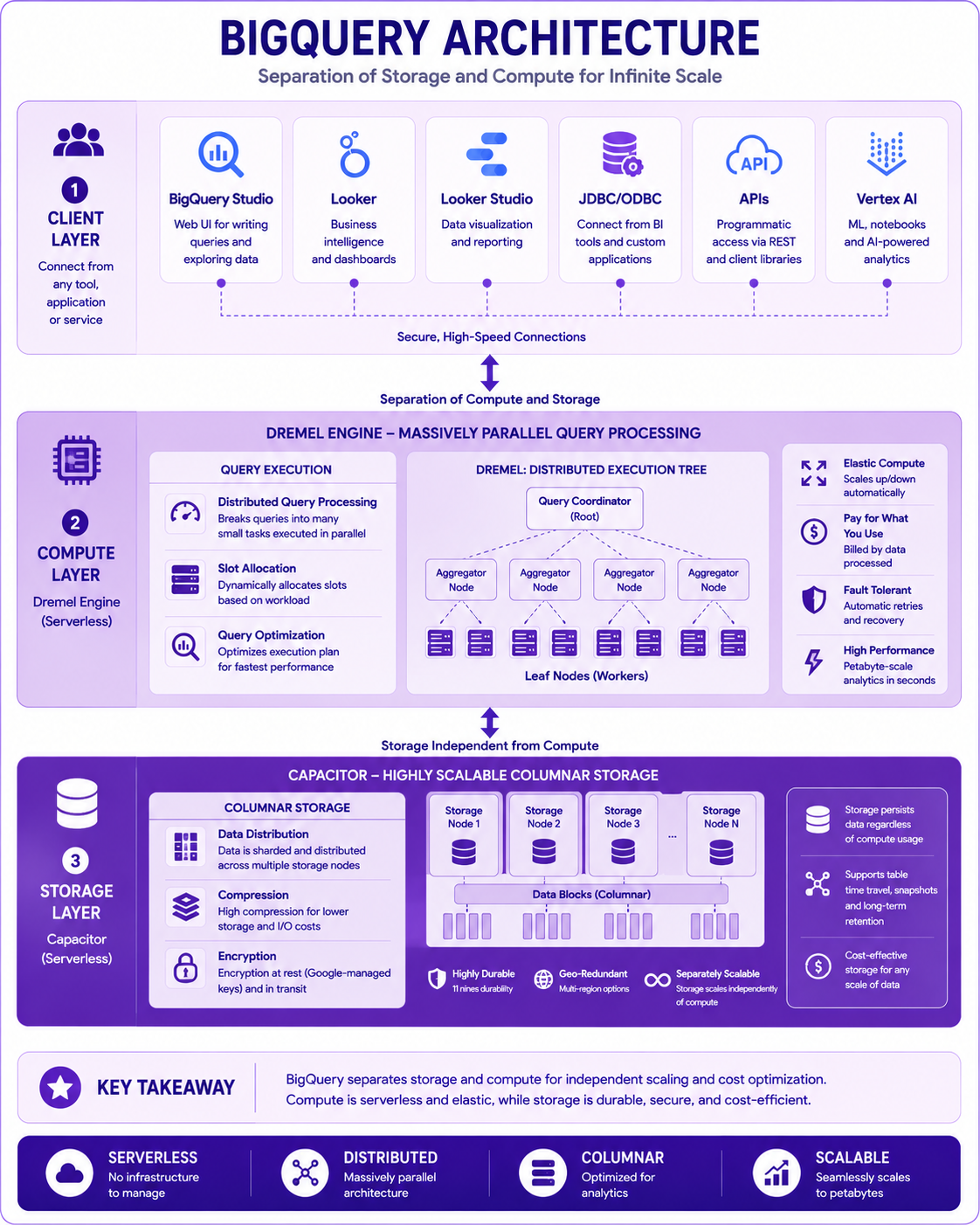
Prompt: Create a comprehensive BigQuery architecture diagram showing the separation of storage and compute. Use a 3-layer structure with purple gradient theme:
Top Layer: Client Layer - Purple #F3E5F5
- BigQuery Studio, Looker, Looker Studio, Vertex AI, JDBC/ODBC, APIs
- Show various connection methods with icons
Middle Layer: Compute Layer (Dremel Engine) - Purple #CE93D8
- Query Execution (Dremel)
- Distributed Query Processing
- Slot Allocation
- Query Optimization
- Show Dremel with distributed execution nodes
Bottom Layer: Storage Layer (Capacitor) - Purple #7B1FA2
- Columnar Storage (Capacitor)
- Data Distribution
- Compression
- Encryption
- Show storage separated from compute
Add large arrows showing separation between compute and storage layers. Include key takeaway at bottom: "BigQuery separates storage and compute for independent scaling and cost optimization." Footer tags: Serverless, Distributed, Columnar, Scalable. Enterprise-style clean layout with rounded corners.
Storage Architecture: Capacitor
Capacitor is BigQuery's proprietary columnar storage format.
Key Characteristics
- Columnar Storage: Data stored by column, not row
- Automatic Compression: High compression ratios
- Encryption: Always encrypted at rest
- Distribution: Data distributed across storage nodes
- Immutability: Data blocks are immutable
- Delta Storage: Updates stored as deltas
Columnar vs Row Storage
| Aspect | Row Storage | Columnar Storage (Capacitor) |
|---|---|---|
| Data Layout | All columns together | Same columns together |
| Query Performance | Good for SELECT * | Excellent for aggregations |
| Compression | Poor | Excellent |
| I/O Efficiency | Reads all columns | Reads only needed columns |
| Update Performance | Good | Moderate |
| Storage Overhead | High | Low |
Columnar Storage Example
Transactional Table (Row Format):
Row 1: [CustID, Name, Age, Balance, LastTransaction, Branch]
Row 2: [CustID, Name, Age, Balance, LastTransaction, Branch]
Row 3: [CustID, Name, Age, Balance, LastTransaction, Branch]

Columnar Format (Capacitor):
Column 1: [CustID1, CustID2, CustID3, ...]
Column 2: [Name1, Name2, Name3, ...]
Column 3: [Age1, Age2, Age3, ...]
Column 4: [Balance1, Balance2, Balance3, ...]
Column 5: [LastTransaction1, LastTransaction2, ...]
Banking Example
-- Query that benefits from columnar storage
SELECT
  branch_id,
  SUM(transaction_amount) as total_volume,
  COUNT(*) as transaction_count
FROM transactions
WHERE transaction_date >= '2024-01-01'
  AND transaction_type = 'PAYMENT'
GROUP BY branch_id;

-- BigQuery only reads:
-- branch_id column, transaction_amount column,
-- transaction_date column, transaction_type column
-- 4 columns instead of all 15+ columns in the table
Compute Architecture: Dremel
Dremel is BigQuery's distributed query execution engine.
Key Characteristics
- Massively Parallel Processing (MPP)
- Distributed Query Execution
- Dynamic Slot Allocation
- Query Optimization
- Result Caching
- Interactive and Batch Modes
Dremel Architecture Components
┌─────────────────────────────────────────────────────────────┐
│                    Dremel Query Engine                       │
├─────────────────────────────────────────────────────────────┤
│  Query Parser & Optimizer                                   │
│  ┌─────────────────────────────────────────────────────┐   │
│  │  - Parse SQL                                        │   │
│  │  - Optimize query plan                              │   │
│  │  - Generate distributed execution plan              │   │
│  └─────────────────────────────────────────────────────┘   │
├─────────────────────────────────────────────────────────────┤
│  Slot Manager                                              │
│  ┌─────────────────────────────────────────────────────┐   │
│  │  - Allocate compute slots                           │   │
│  │  - Manage concurrency                              │   │
│  │  - Balance workload                                │   │
│  └─────────────────────────────────────────────────────┘   │
├─────────────────────────────────────────────────────────────┤
│  Distributed Execution (Shuffle)                           │
│  ┌─────────────────────────────────────────────────────┐   │
│  │  - Distribute work across nodes                     │   │
│  │  - Shuffle data between stages                      │   │
│  │  - Aggregate results                                │   │
│  └─────────────────────────────────────────────────────┘   │
└─────────────────────────────────────────────────────────────┘
BigQuery Architecture Deep Dive
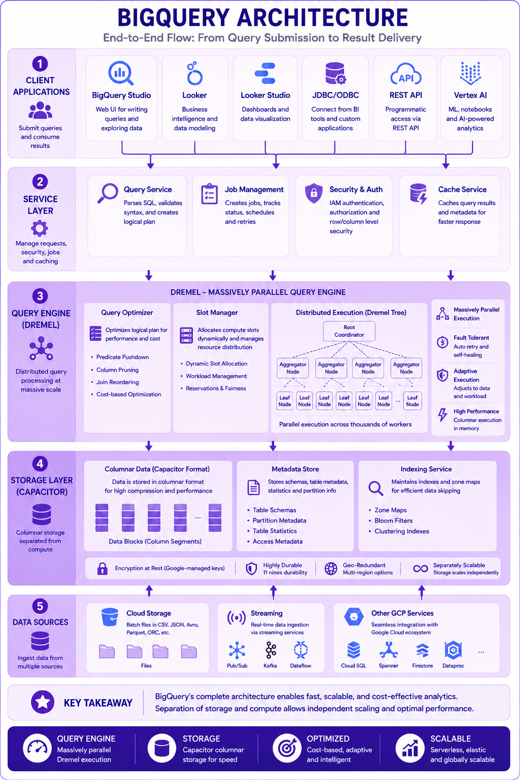
Prompt: Create a detailed BigQuery architecture diagram showing the complete flow from query submission to result delivery. Use a 5-layer structure with purple gradient theme:
Layer 1: Client Applications (Top) - Purple #F3E5F5
- BigQuery Studio, Looker, Looker Studio, JDBC/ODBC, REST API, Vertex AI
- Show icons for each client type
Layer 2: Service Layer - Purple #E1BEE7
- Query Service, Job Management, Security/Auth, Cache Service
- Arrows from clients to service layer
Layer 3: Query Engine (Dremel) - Purple #CE93D8
- Query Optimizer, Slot Manager, Distributed Execution
- Show Dremel's internal components
Layer 4: Storage Layer (Capacitor) - Purple #AB47BC
- Columnar Data, Metadata Store, Indexing Service
- Show storage blocks and metadata
Layer 5: Data Sources (Bottom) - Purple #7B1FA2
- Cloud Storage, Streaming, Other GCP Services
- Show external data sources
Use downward arrows between layers. Include key takeaway at bottom: "BigQuery's complete architecture enables fast, scalable, and cost-effective analytics." Footer tags: Query Engine, Storage, Optimized, Scalable. Enterprise-style clean layout with rounded corners.
Data Distribution and Storage
How BigQuery Stores Data
Data Storage Process:
1. Data is loaded into BigQuery
2. Data is converted to Capacitor format
3. Data is partitioned and distributed
4. Data is compressed and encrypted
5. Data is written to multiple locations
6. Metadata is updated

Distribution Strategy:
- Data distributed across multiple storage nodes
- Each node stores a subset of data
- Queries can parallelize across nodes
- Automatic recovery on node failure
Storage Types
| Storage Type | Description | Use Case |
|---|---|---|
| Active Storage | Frequently accessed data | Recent transactions |
| Long-term Storage | Infrequently accessed data | Historical data (90+ days) |
| Streaming Buffer | Recently ingested data | Real-time data |
Banking Example
Bank Data Distribution:
- Active Storage: Last 3 months transactions (20 TB)
- Long-term Storage: 3-10 years transactions (100 TB)
- Streaming Buffer: Today's transactions (Real-time)

Query Performance:
- Active Storage: Query in 2-5 seconds
- Long-term Storage: Query in 5-15 seconds
- Streaming Buffer: Query in 1-3 seconds
Query Execution Process
Step-by-Step Query Flow
1. Client submits SQL query
   ↓
2. Query Service parses SQL
   ↓
3. Query Optimizer creates execution plan
   ↓
4. Slot Manager allocates compute slots
   ↓
5. Distributed execution across nodes
   ↓
6. Data read from Capacitor storage
   ↓
7. Intermediate results shuffled
   ↓
8. Final aggregation and sorting
   ↓
9. Results returned to client
Query Stages
Stage 1: Query Parsing & Validation
- Syntax check
- Schema validation
- Authorization check

Stage 2: Query Optimization
- Query rewriting
- Join reordering
- Predicate pushdown
- Partition pruning

Stage 3: Distributed Execution
- Sharding data
- Parallel processing
- Intermediate aggregation

Stage 4: Result Assembly
- Shuffle and combine
- Final aggregation
- Return results
Performance Optimization
Partitioning
Partitioning divides a table into segments based on a column.
Partition Types:
- Date/Timestamp Partitioning
- Integer Range Partitioning
- Ingestion Time Partitioning

Benefits:
- Query only relevant partitions
- Faster query execution
- Lower cost
- Better performance
-- Create a partitioned table
CREATE TABLE banking.transactions_partitioned
PARTITION BY DATE(transaction_date)
AS
SELECT * FROM banking.transactions;

-- Query uses partition pruning
SELECT *
FROM banking.transactions_partitioned
WHERE transaction_date BETWEEN '2024-01-01' AND '2024-01-31';
-- Only reads January 2024 partition
Clustering
Clustering organizes data within partitions based on column values.
Clustering Benefits:
- Data is co-located by cluster columns
- Faster filter operations
- Efficient sorting
- Better compression
- Lower query cost
-- Create a clustered table
CREATE TABLE banking.transactions_clustered
PARTITION BY DATE(transaction_date)
CLUSTER BY customer_id, transaction_type
AS
SELECT * FROM banking.transactions;

-- Query benefits from clustering
SELECT *
FROM banking.transactions_clustered
WHERE customer_id = 12345;
-- Data is physically organized by customer_id
Partitioning vs Clustering
| Aspect | Partitioning | Clustering |
|---|---|---|
| Granularity | Coarse | Fine |
| Cardinality | Low (few partitions) | High (many values) |
| Cost | Fixed (per partition) | Variable |
| Performance | Great for date ranges | Great for exact matches |
| When to Use | Date-based queries | Specific value queries |
| Storage Impact | Moderate | Minimal |
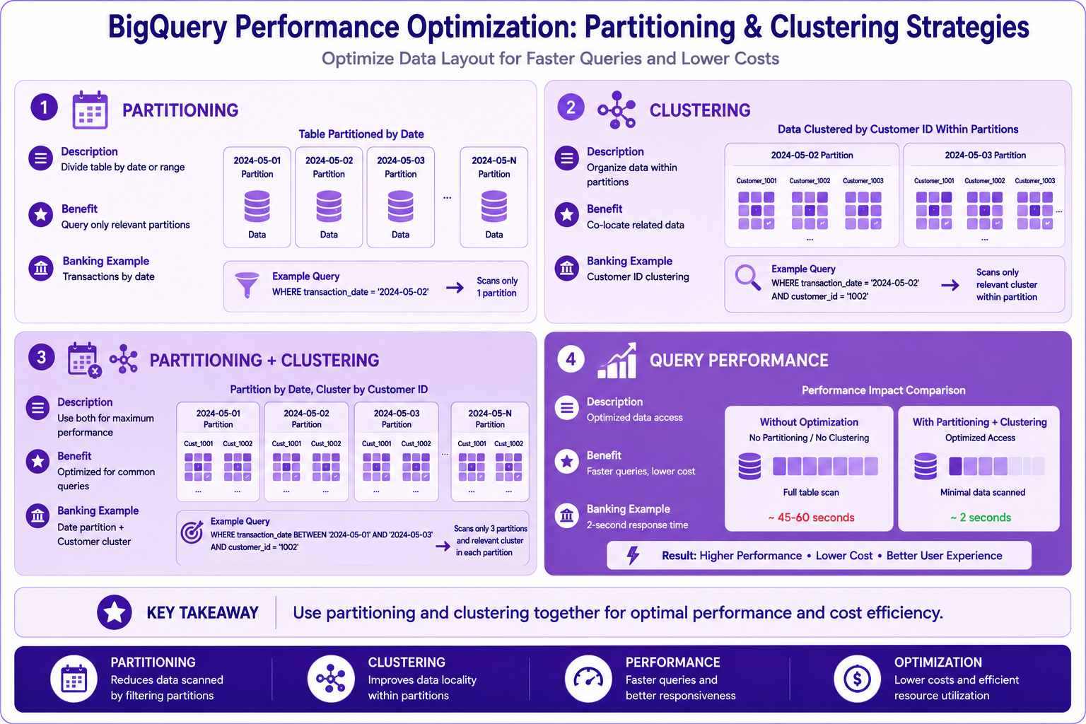
Prompt: Create a performance optimization diagram showing partitioning and clustering strategies. Use a 4-section layout:
Section 1: Partitioning (Top Left) - Purple #F3E5F5
- Icon: 📅 Date/Partition icon
- Title: "Partitioning"
- Description: "Divide table by date or range"
- Benefit: "Query only relevant partitions"
- Banking Example: "Transactions by date"
- Visual: Table divided into date boxes
Section 2: Clustering (Top Right) - Purple #E1BEE7
- Icon: 📊 Cluster icon
- Title: "Clustering"
- Description: "Organize data within partitions"
- Benefit: "Co-locate related data"
- Banking Example: "Customer ID clustering"
- Visual: Data organized within partitions
Section 3: Combined Approach (Bottom Left) - Purple #CE93D8
- Icon: 🔗 Combined icon
- Title: "Partitioning + Clustering"
- Description: "Use both for maximum performance"
- Benefit: "Optimized for common queries"
- Banking Example: "Date partition + Customer cluster"
- Visual: Nested diagram
Section 4: Query Performance (Bottom Right) - Purple #AB47BC
- Icon: ⚡ Performance icon
- Title: "Query Performance"
- Description: "Optimized data access"
- Benefit: "Faster queries, lower cost"
- Banking Example: "2-second response time"
- Visual: Speed comparison
At bottom: Key takeaway: "Use partitioning and clustering together for optimal performance and cost efficiency." Footer tags: Partitioning, Clustering, Performance, Optimization. Enterprise-style clean layout with rounded corners.
Pricing Models
Storage Pricing
Active Storage: ~$0.02 per GB per month
Long-term Storage: ~$0.01 per GB per month (90+ days old)

Banking Example:
- 20 TB Active Storage: $400/month
- 100 TB Long-term Storage: $1,000/month
- Total Storage Cost: $1,400/month
Compute Pricing
- On-demand: $5.00 per TB processed
- Flat-rate: Monthly slots reservation

Banking Example:
- 5,000 queries/day
- Average 10 GB per query
- Daily processed: 50 TB
- Monthly processed: 1,500 TB
- On-demand cost: $7,500/month
- Flat-rate: $2,000/month (saving 73%)
Cost Optimization Strategies
✅ Use partitioning and clustering
✅ Limit data scanned (SELECT only needed columns)
✅ Use materialized views
✅ Implement caching
✅ Use flat-rate for high usage
✅ Set query cost controls
✅ Monitor costs with dashboards
Slot Allocation and Concurrency
What are Slots?
Slots are compute units in BigQuery
- Each slot represents a portion of CPU and memory
- More slots = faster query execution
- Slots are shared across queries
- Slots can be allocated dynamically
Slot Allocation Types
| Type | Description | Use Case |
|---|---|---|
| On-demand | Pay per query | Low volume, variable usage |
| Flat-rate | Reserved slots | Consistent, high volume |
| Flex Slots | Flexible commitment | Variable, predictable patterns |
Concurrency Management
Concurrency Factors:
- Number of queries
- Query complexity
- Data size
- Available slots
- Workload priority

Slot Allocation per Query:
- Simple query: 1-10 slots
- Complex query: 10-100 slots
- Large query: 100-1000 slots
BigQuery Features Deep Dive
BigQuery ML
Build and deploy ML models using SQL
- No data movement
- No additional infrastructure
- SQL-based model training

Banking Examples:
- Credit scoring models
- Customer churn prediction
- Fraud detection models
-- Create a fraud detection model
CREATE OR REPLACE MODEL banking.fraud_detection
OPTIONS(model_type='logistic_reg')
AS
SELECT
  transaction_amount,
  customer_age,
  transaction_frequency,
  is_fraud
FROM banking.transactions_labeled;
BigQuery GIS
Geospatial analytics in BigQuery
- Store and query spatial data
- Geographic analysis
- Location-based insights

Banking Examples:
- Branch performance by location
- ATM optimization
- Market penetration analysis
BigQuery BI Engine
In-memory analysis engine
- Accelerates BI queries
- Sub-second response
- Integration with Looker

Banking Examples:
- Real-time dashboards
- Executive reporting
- Ad-hoc analysis
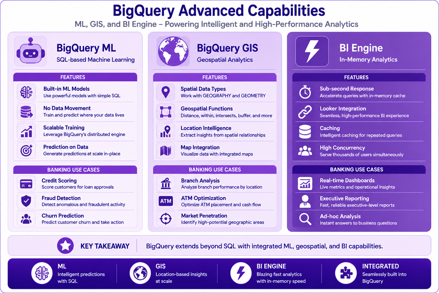
Prompt: Create a BigQuery features diagram highlighting ML, GIS, and BI Engine capabilities. Use a 3-column structure:
Column 1: BigQuery ML (Left) - Purple #E1BEE7
- Title: "BigQuery ML"
- Subtitle: "SQL-based Machine Learning"
- Features: Built-in ML Models, No Data Movement, Scalable Training, Prediction on Data
- Banking Use Cases: Credit Scoring, Fraud Detection, Churn Prediction
- Icon: 🤖 ML icon
Column 2: BigQuery GIS - Purple #CE93D8
- Title: "BigQuery GIS"
- Subtitle: "Geospatial Analytics"
- Features: Spatial Data Types, Geospatial Functions, Location Intelligence, Map Integration
- Banking Use Cases: Branch Analysis, ATM Optimization, Market Penetration
- Icon: 🌍 Map icon
Column 3: BI Engine - Purple #AB47BC
- Title: "BI Engine"
- Subtitle: "In-Memory Analytics"
- Features: Sub-second Response, Looker Integration, Caching, High Concurrency
- Banking Use Cases: Real-time Dashboards, Executive Reporting, Ad-hoc Analysis
- Icon: ⚡ Lightning icon
At bottom: Key takeaway: "BigQuery extends beyond SQL with integrated ML, geospatial, and BI capabilities." Footer tags: ML, GIS, BI Engine, Integrated. Enterprise-style clean layout with rounded corners.
Best Practices
| # | Best Practice |
|---|---|
| 1 | Use partitioning and clustering for performance |
| 2 | SELECT only needed columns to reduce data scan |
| 3 | Use materialized views for frequently used queries |
| 4 | Implement proper data governance |
| 5 | Monitor query performance and costs |
| 6 | Use streaming for real-time data |
| 7 | Implement data retention policies |
| 8 | Use flat-rate pricing for consistent workloads |
| 9 | Set query cost controls |
| 10 | Use caching where appropriate |
Common Mistakes
| # | Common Mistake | Better Approach |
|---|---|---|
| 1 | Not using partitioning | Always partition large tables |
| 2 | Not using clustering | Cluster on frequently queried columns |
| 3 | Using SELECT * | Specify needed columns |
| 4 | No cost controls | Set query budget limits |
| 5 | Unoptimized joins | Design for joins |
| 6 | No monitoring | Monitor performance and costs |
| 7 | Wrong pricing model | Evaluate flat-rate if high volume |
| 8 | Ignoring caching | Use BI Engine for dashboards |
| 9 | No data retention | Implement lifecycle policies |
| 10 | Not using materialized views | Cache expensive queries |
Interview Questions
-
Explain BigQuery's architecture.
-
What is the separation of storage and compute in BigQuery?
-
What is Capacitor and how does it work?
-
What is Dremel and its role in BigQuery?
-
What is the difference between partitioning and clustering?
-
How does BigQuery handle streaming data?
-
Explain BigQuery's pricing model.
-
What are slots and how are they allocated?
-
How does BigQuery ML work?
-
What is BI Engine and when should you use it?
-
How do you optimize query performance in BigQuery?
-
What is the difference between active and long-term storage?
Practice Exercises
-
Create a partitioned table in BigQuery.
-
Create a table with clustering.
-
Write a query that uses partition pruning.
-
Analyze query performance using query plan.
-
Create a materialized view.
-
Implement a streaming pipeline to BigQuery.
-
Set up cost controls and budget alerts.
-
Create a BigQuery ML model.
-
Compare query performance with and without partitioning.
-
Analyze query cost using EXPLAIN.
Key Takeaways
| # | Takeaway |
|---|---|
| 1 | BigQuery separates storage and compute for scalability |
| 2 | Capacitor provides high-performance columnar storage |
| 3 | Dremel enables distributed query execution |
| 4 | Partitioning and clustering optimize performance |
| 5 | Choose appropriate pricing model for cost efficiency |
| 6 | Built-in ML, GIS, and BI Engine extend capabilities |
| 7 | Performance and cost optimization are continuous processes |
| 8 | Monitor and tune queries for best results |
Chapter Summary
In this chapter, you learned:
- ✅ BigQuery's architecture and design principles
- ✅ Capacitor columnar storage format
- ✅ Dremel distributed query engine
- ✅ Data distribution and storage strategies
- ✅ Query execution process
- ✅ Partitioning and clustering optimization
- ✅ Pricing models and cost optimization
- ✅ Slot allocation and concurrency
- ✅ BigQuery ML, GIS, and BI Engine features
- ✅ Best practices and common mistakes
You now have a deep understanding of BigQuery architecture and are ready to implement effective data models.
Next Chapter
👉 Next Chapter: BigQuery Physical Data Modeling