
Chapter 05: BigQuery Physical Data Modeling
In the previous chapter, we explored BigQuery's architecture and learned how its separation of storage and compute enables scalable analytics.
In this chapter, we will learn how to design physical data models in BigQuery, optimize table structures, implement partitioning and clustering strategies, and apply best practices for performance and cost efficiency.
Using our Digital Banking Platform case study, we will create optimized physical data models that support real-world banking analytics.
🎯 Learning Objectives
By the end of this chapter, you will be able to:
- Understand BigQuery physical data modeling concepts
- Design optimized table structures
- Implement effective partitioning strategies
- Apply clustering for query performance
- Choose appropriate data types
- Understand table lifecycle management
- Optimize for cost and performance
- Implement best practices for physical modeling
What is Physical Data Modeling?
Physical data modeling is the process of translating logical data models into optimized database structures that deliver the best performance and cost efficiency for specific query patterns.
Conceptual Model (Business View)
         ↓
Logical Model (Relationships)
         ↓
Physical Model (Optimized Storage)
         ↓
BigQuery Implementation
Think of physical modeling as:
- Deciding how data is stored physically
- Choosing storage formats
- Designing for query patterns
- Optimizing for performance
- Managing cost efficiency
Real-World Banking Example
A bank needs to optimize its transaction data for analytics:
Business Requirement:
- Query transaction history for 50 million customers
- Support real-time fraud detection
- Generate daily regulatory reports
- Analyze 10+ years of transaction data

Logical Model:
- Transaction table with 20+ columns
- Foreign keys to customer, account, branch

Physical Optimization:
- Partition by transaction_date
- Cluster by customer_id
- Use appropriate data types
- Implement lifecycle policies
BigQuery Table Types
Native Tables
Description: Standard BigQuery managed tables
Use Case: Most analytical workloads
Characteristics:
- Fully managed by BigQuery
- Automatic optimization
- Supports partitioning and clustering
- Columnar storage (Capacitor)
External Tables
Description: Tables that reference data in external sources
Use Case: Querying data in Cloud Storage, Cloud Drive, etc.
Characteristics:
- No data stored in BigQuery
- Query data at source
- Supports partitioning
- Limited performance
Materialized Views
Description: Pre-computed query results stored as tables
Use Case: Frequently used aggregations and joins
Characteristics:
- Automatically refreshed
- Query rewrite benefits
- Cost savings on repeated queries
- Supports incremental refresh
Temporary Tables
Description: Session-scoped tables
Use Case: Intermediate query results
Characteristics:
- Session lifespan
- No permanent storage
- Not shareable
- Good for ETL pipelines
Table Design Best Practices
1. Choose the Right Data Types
| Data Type | Banking Example | Size | Best Practice |
|---|---|---|---|
| INT64 | Customer ID | 8 bytes | Use for numeric IDs |
| STRING | Customer Name | Variable | Use for text fields |
| TIMESTAMP | Transaction Time | 8 bytes | Use for date/time |
| DATE | Transaction Date | 4 bytes | Use for partitioning |
| NUMERIC | Transaction Amount | 16 bytes | Use for financial amounts |
| BOOLEAN | Is Fraudulent | 1 byte | Use for flags |
| STRUCT | Address | Variable | Use for related fields |
2. Use Appropriate Data Types
-- Example: Optimized transaction table
CREATE OR REPLACE TABLE banking.transactions_optimized (
  transaction_id STRING NOT NULL,      -- VARCHAR-like
  customer_id INT64 NOT NULL,           -- Optimized for joins
  account_id INT64 NOT NULL,            -- Optimized for joins
  transaction_date DATE NOT NULL,       -- Partition key
  transaction_timestamp TIMESTAMP,      -- For time-based analysis
  transaction_amount NUMERIC(15,2),     -- Financial precision
  transaction_type STRING,              -- Categorical
  merchant_category STRING,             -- Categorical
  is_fraud BOOLEAN,                     -- Efficient storage
  location STRUCT<                     -- Semi-structured
    latitude FLOAT64,
    longitude FLOAT64,
    country STRING,
    city STRING
  >,
  payment_method STRING,                -- Categorical
  currency_code STRING                 -- Categorical
)
PARTITION BY DATE(transaction_date)
CLUSTER BY customer_id, transaction_type;
3. Minimize Repeated Fields
-- Bad: Repeated fields as array
CREATE TABLE transactions_bad (
  transaction_id STRING,
  transaction_amounts ARRAY<NUMERIC>,  -- Inefficient
  transaction_dates ARRAY<DATE>        -- Hard to query
);

-- Good: Normalized structure
CREATE TABLE transactions_good (
  transaction_id STRING,
  transaction_amount NUMERIC,
  transaction_date DATE
);
4. Use STRUCT for Related Fields
-- Good: Using STRUCT for location
CREATE TABLE transactions_with_location (
  transaction_id STRING,
  location STRUCT<
    latitude FLOAT64,
    longitude FLOAT64,
    country STRING,
    city STRING,
    postal_code STRING
  >
);

-- Query example
SELECT
  transaction_id,
  location.city,
  location.country
FROM transactions_with_location;
Partitioning Strategies
Date Partitioning
-- Best for time-based analytics
CREATE TABLE banking.transactions_date_partitioned
PARTITION BY DATE(transaction_date)
AS
SELECT * FROM banking.transactions;
Ingestion Time Partitioning
-- Automatically partitions by ingestion time
CREATE TABLE banking.transactions_ingestion_partitioned
PARTITION BY _PARTITIONDATE
AS
SELECT * FROM banking.transactions;
Integer Range Partitioning
-- Best for numeric range queries
CREATE TABLE banking.customer_segments
PARTITION BY RANGE_BUCKET(age, GENERATE_ARRAY(18, 100, 10))
AS
SELECT * FROM banking.customers;
Partitioning Best Practices
| Practice | Description |
|---|---|
| Partition Size | Aim for 10-100 GB per partition |
| Partition Count | Max 4,000 partitions per table |
| Partition Key | Use DATE/TIMESTAMP or INTEGER |
| Query Performance | Always filter by partition key |
| Cost Efficiency | Only scan required partitions |
Clustering Strategies
Single Column Clustering
-- Cluster by a single column
CREATE TABLE banking.transactions_clustered_customer
PARTITION BY DATE(transaction_date)
CLUSTER BY customer_id
AS
SELECT * FROM banking.transactions;

-- Query optimized for customer lookups
SELECT *
FROM banking.transactions_clustered_customer
WHERE customer_id = 12345;
-- Data is physically organized by customer_id
Multiple Column Clustering
-- Cluster by multiple columns
CREATE TABLE banking.transactions_clustered_multiple
PARTITION BY DATE(transaction_date)
CLUSTER BY customer_id, transaction_type, merchant_category
AS
SELECT * FROM banking.transactions;

-- Query uses clustering columns
SELECT *
FROM banking.transactions_clustered_multiple
WHERE customer_id = 12345
  AND transaction_type = 'PAYMENT'
  AND merchant_category = 'RETAIL';
Clustering Best Practices
| Practice | Description |
|---|---|
| Column Order | Most frequently filtered first |
| Column Count | Limit to 4-5 columns |
| Cardinality | Balance high vs low cardinality |
| NULL Values | Avoid columns with many NULLs |
| Update Frequency | Consider how often data changes |
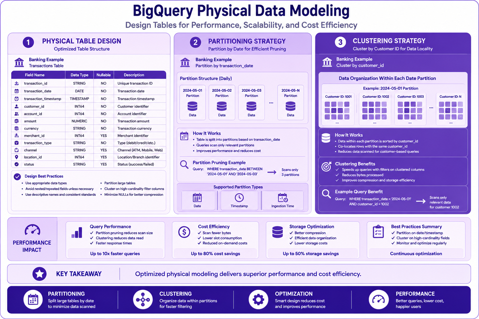
Prompt: Create a comprehensive BigQuery physical data modeling diagram showing table structure, partitioning, and clustering. Use a 3-section layout with purple gradient theme:
Section 1: Table Structure (Left) - Purple #F3E5F5
- Title: "Physical Table Design"
- Show optimized table structure with fields
- Include data types, nullable, description
- Banking Example: "Transactions Table"
- Visual: Table columns with types
Section 2: Partitioning (Middle) - Purple #CE93D8
- Title: "Partitioning Strategy"
- Show partition by date
- Include partition structure
- Banking Example: "Partition by transaction_date"
- Visual: Date-based partitions
Section 3: Clustering (Right) - Purple #7B1FA2
- Title: "Clustering Strategy"
- Show cluster by customer_id
- Include data organization
- Banking Example: "Cluster by customer_id"
- Visual: Data organized by cluster key
Bottom Section: Performance Metrics - Purple #AB47BC
- Query Performance
- Cost Efficiency
- Storage Optimization
- Best Practices Summary
At bottom: Key takeaway: "Optimized physical modeling delivers superior performance and cost efficiency." Footer tags: Partitioning, Clustering, Optimization, Performance. Enterprise-style clean layout with rounded corners and consistent iconography.
Data Lifecycle Management
Table Expiration
-- Set expiration for temporary tables
CREATE TABLE banking.temp_transactions
OPTIONS(expiration_timestamp=TIMESTAMP_ADD(CURRENT_TIMESTAMP(), INTERVAL 7 DAY))
AS
SELECT * FROM banking.transactions
WHERE transaction_date > DATE_SUB(CURRENT_DATE(), INTERVAL 7 DAY);
Partition Expiration
-- Automatically expire old partitions
CREATE TABLE banking.transactions_partition_expired
PARTITION BY DATE(transaction_date)
OPTIONS(
  partition_expiration_days=365,  -- 1 year retention
  require_partition_filter=true    -- Force partition filtering
)
AS
SELECT * FROM banking.transactions;
Time Travel and Storage
-- Query historical data (7 day default)
SELECT * FROM banking.transactions
FOR SYSTEM_TIME AS OF TIMESTAMP_SUB(CURRENT_TIMESTAMP(), INTERVAL 2 DAY);

-- Restore from time travel
CREATE OR REPLACE TABLE banking.transactions
AS
SELECT * FROM banking.transactions
FOR SYSTEM_TIME AS OF TIMESTAMP_SUB(CURRENT_TIMESTAMP(), INTERVAL 2 DAY);
Schema Evolution
Adding New Columns
-- Add new column
ALTER TABLE banking.transactions
ADD COLUMN risk_score INT64;

-- Add column with default
ALTER TABLE banking.transactions
ADD COLUMN risk_level STRING
OPTIONS(description = 'Risk level based on transaction pattern');
Modifying Column Definitions
-- Change column description
ALTER TABLE banking.transactions
ALTER COLUMN transaction_amount
SET OPTIONS(description = 'Amount in USD');

-- Change column mode (requires recreation)
-- RECREATE TABLE with new definition
CREATE OR REPLACE TABLE banking.transactions
AS
SELECT
  transaction_id,
  customer_id,
  account_id,
  transaction_date,
  transaction_amount,
  -- New column
  CASE
    WHEN transaction_amount < 100 THEN 'SMALL'
    WHEN transaction_amount < 1000 THEN 'MEDIUM'
    ELSE 'LARGE'
  END AS transaction_size
FROM banking.transactions_original;
Renaming Columns
-- Rename column (requires recreation)
CREATE OR REPLACE TABLE banking.transactions
AS
SELECT
  transaction_id,
  customer_id,
  account_id,
  transaction_date,
  transaction_amount AS amount,  -- Renamed
  transaction_type
FROM banking.transactions_original;
Query Optimization Techniques
Use Column Filtering
-- Bad: Select all columns
SELECT * FROM banking.transactions WHERE transaction_date = '2024-01-01';

-- Good: Select only needed columns
SELECT
  transaction_id,
  customer_id,
  transaction_amount,
  merchant_category
FROM banking.transactions
WHERE transaction_date = '2024-01-01';
Use Partition Pruning
-- Bad: No partition filter
SELECT *
FROM banking.transactions
WHERE transaction_date > '2024-01-01';  -- Still prunes if using DATE

-- Good: Direct partition filter
SELECT *
FROM banking.transactions
WHERE transaction_date = '2024-01-01';  -- Only one partition
Use Approximate Queries
-- Approximate count for large datasets
SELECT APPROX_COUNT_DISTINCT(customer_id) as unique_customers
FROM banking.transactions
WHERE transaction_date >= DATE_SUB(CURRENT_DATE(), INTERVAL 30 DAY);

-- Approximate quantiles
SELECT
  APPROX_QUANTILES(transaction_amount, 10) as amount_percentiles
FROM banking.transactions;
Materialized Views
Creating Materialized Views
-- Daily transaction summary
CREATE MATERIALIZED VIEW banking.daily_transaction_summary
AS
SELECT
  DATE(transaction_date) as date,
  customer_id,
  COUNT(*) as transaction_count,
  SUM(transaction_amount) as total_amount,
  AVG(transaction_amount) as avg_amount
FROM banking.transactions
GROUP BY DATE(transaction_date), customer_id;

-- Query automatically uses materialized view
SELECT *
FROM banking.daily_transaction_summary
WHERE date = '2024-01-01';
Materialized View Best Practices
| Practice | Description |
|---|---|
| Aggregation | Use for sums, counts, averages |
| Joins | Consider for denormalized views |
| Refresh | Automatic or manual refresh |
| Cost | Storage cost vs query cost |
| Staleness | Acceptable data age |
Cost Optimization with Physical Modeling
Query Cost Reduction
-- Bad: Expensive query
SELECT *
FROM banking.transactions
WHERE DATE(transaction_date) = '2024-01-01';  -- Function on column

-- Good: Efficient query
SELECT *
FROM banking.transactions
WHERE transaction_date >= '2024-01-01'
  AND transaction_date < '2024-01-02';  -- Direct date range
Storage Cost Optimization
-- Optimize storage with appropriate data types
CREATE OR REPLACE TABLE banking.transactions_optimized
PARTITION BY DATE(transaction_date)
CLUSTER BY customer_id
AS
SELECT
  CAST(transaction_id AS STRING) AS transaction_id,
  CAST(customer_id AS INT64) AS customer_id,  -- Smaller
  CAST(account_id AS INT64) AS account_id,    -- Smaller
  CAST(transaction_amount AS NUMERIC(15,2)) AS transaction_amount,
  CAST(transaction_date AS DATE) AS transaction_date,
  CAST(transaction_type AS STRING) AS transaction_type
FROM banking.transactions;
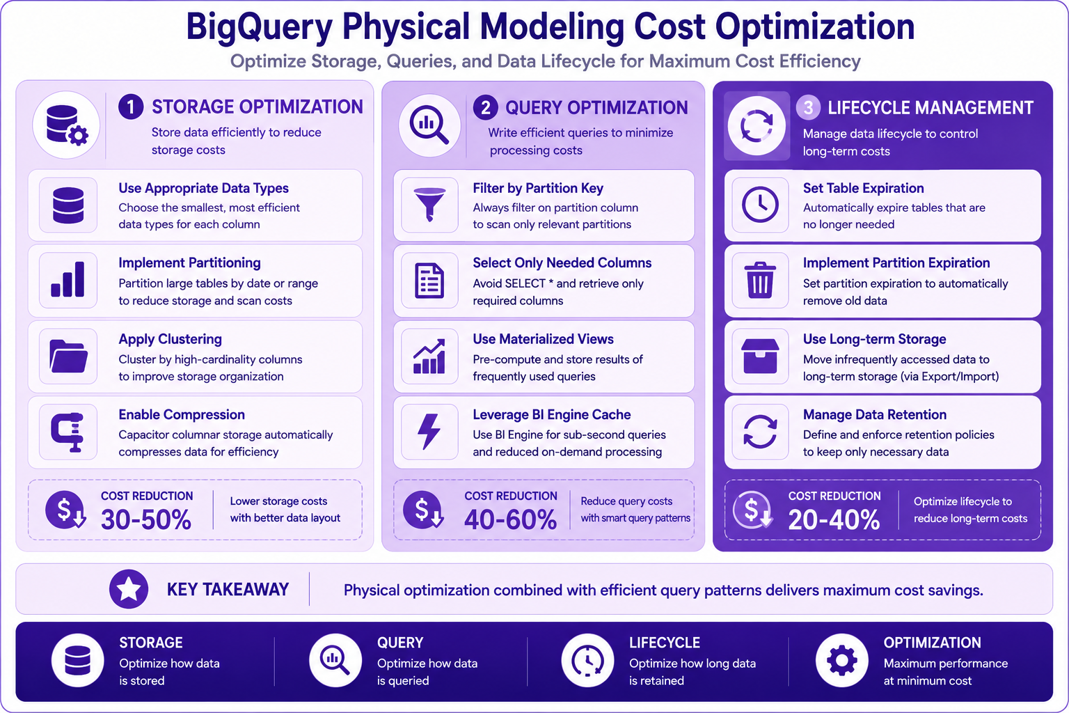
Prompt: Create a cost optimization diagram for BigQuery physical modeling. Use a 3-column structure with purple gradient theme:
Column 1: Storage Optimization (Left) - Purple #E1BEE7
- Title: "Storage Optimization"
- 💾 Use Appropriate Data Types
- 📊 Implement Partitioning
- 🗂️ Apply Clustering
- 🗜️ Enable Compression
- 💰 Cost Reduction: 30-50%
Column 2: Query Optimization - Purple #CE93D8
- Title: "Query Optimization"
- 🔍 Filter by Partition Key
- 📋 Select Only Needed Columns
- 📈 Use Materialized Views
- ⚡ Leverage BI Engine Cache
- 💰 Cost Reduction: 40-60%
Column 3: Lifecycle Management - Purple #AB47BC
- Title: "Lifecycle Management"
- ⏰ Set Table Expiration
- 🗑️ Implement Partition Expiration
- 📦 Use Long-term Storage
- 🔄 Manage Data Retention
- 💰 Cost Reduction: 20-40%
At bottom: Key takeaway: "Physical optimization combined with efficient query patterns delivers maximum cost savings." Footer tags: Storage, Query, Lifecycle, Optimization. Enterprise-style clean layout with rounded corners and consistent iconography.
Best Practices
| # | Best Practice |
|---|---|
| 1 | Use appropriate data types for each column |
| 2 | Always partition large tables |
| 3 | Cluster on frequently filtered columns |
| 4 | Use materialized views for common aggregations |
| 5 | Set table and partition expiration |
| 6 | Implement require_partition_filter |
| 7 | Use STRUCT for related fields |
| 8 | Minimize repeated fields |
| 9 | Consider cost in query design |
| 10 | Monitor and optimize continuously |
Common Mistakes
| # | Common Mistake | Better Approach |
|---|---|---|
| 1 | Using STRING for all text fields | Use appropriate type (INT64, DATE) |
| 2 | No partitioning on large tables | Always partition large tables |
| 3 | Over-clustering (too many columns) | Limit to 4-5 columns |
| 4 | Using SELECT * in production | Select only needed columns |
| 5 | No partition expiration | Set appropriate retention |
| 6 | Not using materialized views | Cache common aggregations |
| 7 | Ignoring cost implications | Monitor and optimize |
| 8 | Over-normalizing for analytics | Use denormalized structures |
| 9 | Not using STRUCT for related data | Use STRUCT for organization |
| 10 | No data lifecycle management | Plan for data growth |
Interview Questions
-
What is physical data modeling in BigQuery?
-
Explain partitioning strategies in BigQuery.
-
How does clustering work in BigQuery?
-
What are the different table types in BigQuery?
-
When would you use a materialized view?
-
How do you optimize BigQuery tables for performance?
-
Explain the difference between partitioning and clustering.
-
What are the best practices for BigQuery physical modeling?
-
How do you manage data lifecycle in BigQuery?
-
What is the impact of data types on storage and performance?
-
How do you design for cost optimization in BigQuery?
-
What is partition expiration and when should you use it?
Practice Exercises
-
Create a partitioned table for banking transactions.
-
Create a clustered table on customer_id.
-
Implement partition expiration for 2 years of data.
-
Create a materialized view for daily transaction summaries.
-
Optimize a table with appropriate data types.
-
Implement require_partition_filter on a table.
-
Add a new column to an existing table.
-
Compare query performance with and without partitioning.
-
Implement a table with STRUCT fields.
-
Set up a data lifecycle management strategy.
Key Takeaways
| # | Takeaway |
|---|---|
| 1 | Physical modeling optimizes storage and query performance |
| 2 | Partitioning reduces data scanned and improves performance |
| 3 | Clustering organizes data for efficient filtering |
| 4 | Choose appropriate data types for storage efficiency |
| 5 | Materialized views cache common aggregations |
| 6 | Data lifecycle management controls costs |
| 7 | Design with query patterns in mind |
| 8 | Balance performance, cost, and maintainability |
Chapter Summary
In this chapter, you learned:
- ✅ Physical data modeling concepts in BigQuery
- ✅ Table types and their use cases
- ✅ Partitioning strategies and best practices
- ✅ Clustering strategies and best practices
- ✅ Data type selection and optimization
- ✅ Data lifecycle management
- ✅ Materialized views and their benefits
- ✅ Cost optimization techniques
- ✅ Best practices and common mistakes
You now have the skills to design optimized physical data models in BigQuery.
Next Chapter
👉 Next Chapter: Lakehouse Architecture